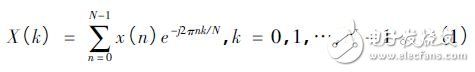
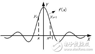
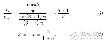
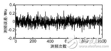
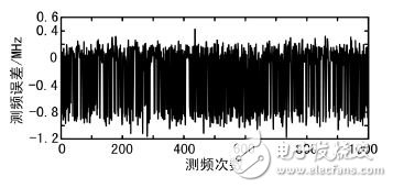
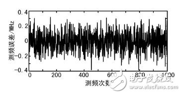
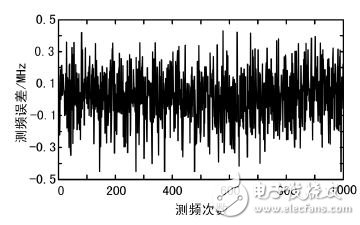
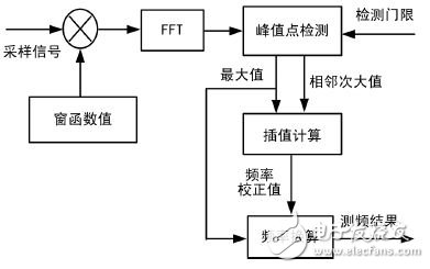
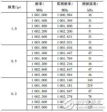
Pulse signal is the main form of signal used by modern radar. Pulse signal frequency measurement is an indispensable part of radar reconnaissance and plays an important role in radar confrontation. Digital processing is one of the trends in the development of radar countermeasure systems. Commonly used digital frequency measurement methods include zero-crossing detection, phase difference method, fast Fourier transform (FFT) method and modern spectrum estimation method. Among them, FFT method engineering has strong realizability, good real-time performance, and is suitable for broadband detection, so it is widely used in engineering. In this paper, the sinusoidal pulse signal with short time width (0. 2 ~ 1 μs) is taken as the research object. The shortcomings of the traditional FFT frequency measurement method are analyzed. The improved method of improving the frequency measurement accuracy is analyzed from the perspective of engineering application. An FPGA-based all-digital implementation process is proposed. The signal x( t) is digitally sampled as x( n) , n = 0,1,2,...,N - 1 for spectral analysis, discrete Fourier transform (DFT), and signal from time to time The domain is converted to the frequency domain as shown in equation (2): The fast algorithm used in DFT implementation is FFT. After FFT processing, the frequency resolution of the signal is: Where fs is the sampling rate, and the time width of the signal is T, then the number of points of the signal is T &TImes; fs, the frequency resolution of the signal can be expressed as: It can be seen that the frequency resolution of the FFT frequency measurement is only related to the signal time width, and the frequency of the signal is converted according to the maximum value of the spectral line. If the frequency of the signal falls on a line, the obtained frequency measurement result is accurate. In most cases, the signal frequency falls between the two spectral lines, and the frequency reflected by the maximum spectral line position is no longer accurate. The maximum frequency error is Δf /2 . Pulse is the most commonly used form of radar. If necessary, the radar sometimes uses the pulse-modulated signal type, such as phase encoding, linear frequency modulation, etc. For such complex signals, various signal processing methods can be used to convert it into ordinary signals. The sine wave signal, therefore the frequency measurement method of the sine wave pulse is versatile. According to the above analysis results, for the pulse with longer time width, the FFT frequency measurement method is easy to achieve higher frequency measurement accuracy and meet the requirements of equipment specifications. However, for short pulses, such as a pulse of 0.2 μs wide, according to equation (3), the theoretically achievable frequency measurement accuracy is only 2. 5 MHz, which is difficult to meet the reconnaissance requirements. Zero padding is the addition of zeros at the end of the time domain data before the FFT operation, and keeping the total time domain data points at a power of two. Since zero padding does not add any new information, it does not change the spectral shape and frequency resolution. Zero padding only interpolates some frequency components in the FFT result of the original point number. For FFT results with fewer points, in most cases, it is difficult to find the peaks, and it is difficult to observe the fine structure of the spectrum. After the zero padding, the peak position of the power spectrum can be clearly displayed, which helps to improve the ability to accurately locate the peak frequency component of the main lobe, thereby improving the frequency measurement accuracy. The disadvantage of zero-padding technology is that it increases the amount of processing. The more zero-padding, the longer the processing time. In addition, in the case of noise, zero-padding can not improve the signal-to-noise ratio, and there is a possibility that the spectral peak point is located incorrectly, resulting in an increase in the frequency measurement error. 3. 1 Interpolated FFT frequency estimation principle The interpolated FFT estimation frequency method uses two FFT lines on both sides of the true spectral peak to find the amplitude ratio, establish an equation with the modified frequency as the variable, solve the equation to obtain the corrected frequency value, and correct the FFT maximum line position. To achieve a more accurate estimate of the signal frequency, as shown in Figure 1. Compared to the method of zero padding in the previous section, it is not necessary to increase the length of the FFT and the amount of computational processing that comes with it. It is sufficient to find two points from the FFT result. Figure 1 rectangular window spectrum function In Figure 1, the interpolation frequency correction is used to find the difference between the center of the main lobe of the rectangular window spectrum and the adjacent line. For the line position x, x + 1, the rectangular window function is sinc, which is expressed as f(x). ), the spectral values ​​are yx, yx+1, the rectangular window spectrum function and the spectral value are known, and an equation can be constructed as follows: In Figure 1, the sinc function has a peak abscissa of zero and a frequency correction value of δ = - x . As long as x is solved according to equation (4), the frequency correction value can be obtained. Normalize the rectangular window spectral function, and obtain the modulus: Bring in (4) and get: Where α = yx /yx+1 . In practical applications, the FFT peak maximum position k1, the adjacent sub-large value position k2, and the frequency resolution Δf are known, and the corrected frequency value is used to correct the frequency: When k2 = k1 + 1, take the plus sign; when k2 = k1 - 1, take the minus sign. 3. 2 performance analysis under noise conditions The theoretical analysis of the interpolated FFT frequency estimation method is carried out. In practical applications, there will inevitably be background noise. This section will analyze the performance of the interpolated FFT frequency estimation method in the context of additive white Gaussian noise. Set the simulation parameters, the signal sampling rate fs is 1 280 MHz, the pulse width is 0.2 μs, the frequency is set to f1 to 102. 4 MHz, and f2 is 100. 4 MHz, and Gaussian white noise is added according to the signal-to-noise ratio of 10 dB. The simulation is performed at the signal frequency f1, and the frequency is continuously measured 1000 times. The simulation results are shown in Fig. 2. As can be seen from the figure, the maximum frequency error does not exceed 300 kHz. Figure 2 Frequency measurement error map The simulation is carried out at the signal frequency f2, and the frequency is continuously measured 1000 times. The simulation results are shown in Fig. 3. As can be seen from Figure 3, the maximum frequency error exceeds 1 MHz. Figure 3 frequency error variation diagram It is easy to know from the above results that the interpolation frequency measurement error in the noise background is related to the selection of the frequency position. To be precise, it is the distance from the actual frequency position away from the FFT spectrum, that is, the frequency correction value δ. In general, the FFT amplitude maximum value k1 and the adjacent sub-large value k2 are located in the main lobe of the rectangular window function. When the actual frequency position is near the middle of k1 and k2, the signal leaks more energy to both sides. Under the signal-to-noise ratio, the k1 and k2 are electrically averaged larger than the noise level, ensuring that the k2 position is not misplaced, which corresponds to the situation in Figure 2. When the δ value is close to 0, more signal energy is concentrated at k1, and the amplitude at k2 is smaller, and the amplitude k3 of the other side of the largest spectral line is affected by noise, which is close to the amplitude of k2, thus causing the maximum. The position of the next largest spectral line adjacent to the line is misplaced, resulting in the addition or subtraction of the symbol error in equation (7), which causes a large error in the frequency measurement result, corresponding to the situation in FIG. It can be seen that in the noise background, the interpolation FFT frequency measurement method has limitations, that is, only when the δ value is greater than a certain threshold value, the ideal frequency measurement accuracy can be achieved. 3. 3 windowing performance analysis To suppress spectral leakage, the sampled data is often windowed before the FFT. While suppressing the leak, windowing will widen the main lobe of the spectrum. For the interpolation FFT method to find the frequency, regardless of the spectral maximum deviation from the actual FFT line distance, the maximum value and its adjacent two spectral lines are included in the main lobe. Under certain SNR conditions, the next largest value is not It will approach the noise level, making the anti-noise performance enhanced. After windowing, the frequency correction value still varies with the magnitude of k1 and k2, but the variation law is no longer based on the sinc function. The frequency correction calculation formula corresponding to several window functions is given in [7]. When selected, the calculation formula is easier to implement. . Adding a Hanning window to the sampled data, using the ratio α of k1 and k2 to bring into the window function, can be derived by: The analytical formula for estimating the frequency correction value δ using α is as follows: The method of correcting the frequency is shown in equation (10). The simulation parameters are set, the signal sampling rate and the pulse width are unchanged, and Gaussian white noise is still added according to the signal-to-noise ratio of 10 dB. The continuous frequency measurement is 1000 times. The simulation result of frequency f1 is shown in Fig. 4. The simulation result of frequency f2 is shown in Fig. 5. Figure 4 Frequency measurement error map Figure 5 frequency error variation diagram It can be seen from the simulation results that the maximum frequency error does not exceed 500 kHz. After windowing, under the condition of conventional signal-to-noise ratio, the probability of sub-large value direction error is greatly reduced, and the resulting frequency estimation error can be neglected. The block diagram of the implementation of the Jia Hanning window interpolation FFT frequency measurement is shown in Figure 6. The whole algorithm can be implemented in one FPGA. After the sampled data enters the FPGA, it is multiplied by the Hanning window value. The Hanning window value can be pre-stored in the ROM of the FPGA and read out in a table lookup mode. The windowed data enters the FFT module for pipeline processing to obtain the spectrum result of the signal, and performs peak search on the spectrum result, and compares it with the detection threshold to determine whether there is a signal. When the spectrum peak is greater than the detection threshold, the peak position is found adjacent. The spectral position of the larger amplitude is interpolated and converted according to equation (8) to obtain the frequency estimation value. Figure 6 Windowed interpolation FFT frequency measurement implementation block diagram In the formula (10), there is a division calculation. In the implementation, the division can be converted into a process of first reciprocal of the divisor and then multiplying by the dividend. The rich RAM resources in the FPGA are used to calculate the inverse calculation using the look-up table. In addition, the operation is only composed of regular addition and multiplication, which is convenient for FPGA implementation. For a broadband reconnaissance receiver, the indicator requires adaptation to a pulse width of 0.2 to 1 000 μs and a frequency error of no more than 500 kHz. The implementation of the signal detection and frequency measurement is done by the FPGA hardware, the algorithm is implemented by a fixed point, and the resolution of the frequency is set to 15.625 kHz. The frequency measurement result is sent to the software display, and the error unit is kHz, which is rounded. The signal amplitude is set to be 3 dB above the measured sensitivity of the receiver, and the frequency is selected from 1 001 to 1 003 MHz and 200 kHz steps, and the pulse width is set to 1 μs, 0.5 μs, and 0.2 μs, respectively. The test results are shown in Table 1. Table 1 Radar signal frequency measurement accuracy test results It can be seen that the maximum error of the frequency measurement is less than 500 kHz at different frequencies and different pulse widths, which meets the requirements of the index. 6 Conclusion A real-time frequency measurement algorithm for pulse signals that is easy to implement is discussed. Compared with the traditional method, higher frequency measurement accuracy can be achieved. It has been proved by experiments that it can meet the requirements of the current conventional radar reconnaissance receivers and can be applied to electronic countermeasure systems with pulse signals. It has high application value.
PLC splitter is a type of optical power management device that is fabricated using silica optical waveguide technology. It features small size, high reliability, wide operating wavelength range and good channel-to channel uniformity, and is widely used in PON networks to realize optical signal power splitting.
Bwinners provides whole series of 1×N and 2×N splitter products that are tailored for specific applications. All products meet GR-1209-CORE and GR-1221-CORE requirements. Fiber Optic Splitter Plc, Fiber Optic Cable Splitter, Optical Splitter, Mini Type Plc Splitter, Cassette Type Plc Splitter, Insertion Module Plc are available.
Features:
Low insertion loss and low PDL
Fiber Optical communication system
Fiber Optical access networks
Fiber Sensor Cassette Fiber Plc Splitter,Gpon Splitter Cassette,Plc Splitter Cassette Box,Optical Splitter Cassette Type Sijee Optical Communication Technology Co.,Ltd , https://www.sijee-optical.com
Various coupling ratio
Environment stable
Single mode and multimode available
High Reliability and Stability
High Channel counts
Wide wavelength range
Customized packaging and configuration
Applications:
FTTx Construction
Fiber CATV networks
Local area networks